Linear Programming
This note is part of my learning notes on Data Structures & Algorithms.
Linear Programming
Linear programming is an optimization technique for a system of linear constraints and a linear objective function. An objective function defines the quantity to be optimized, and the goal of linear programming is to find the values of the variables that maximize or minimize the objective function.
Formal Definition
Given:
- number of Real-value variables
- Linear objective function
- number of Linear inequalities (constraints)
is an matrix
Goal: Find values for all that satisfy the constraints and maximize / minimize the objective function.
Simple Example of a LP problem
Given a max (objective function) , subjected to (s.t.) constraints:
Find the values of and , so that has a max value.
Simplex Method
Simplex method is an algorithm used to solve linear programming problems.
Given the objective function and inequality constraints,
- Convert the inequalities into equations by adding one slack variable for each inequality
Construct the initial simplex tableau
The most negative entry in the bottom row identifies the pivot column.
https://math.libretexts.org/Bookshelves/Applied_Mathematics/Applied_Finite_Mathematics_(Sekhon_and_Bloom)/04%3A_Linear_Programming_The_Simplex_Method/4.02%3A_Maximization_By_The_Simplex_Method
Now we’ll use linear programming to model some algorithm problems.
Example: Max-Flow
Find the max flow in from source node to sink node .
Capacity constraint:
Because the capacity constraints and flow conservation rule of the flow network can be used as the constraints for linear programming. Hence, we model it with linear programming.
Example: Min-Cost Max Flow
- Ignore cost, get max flow
Example: L1 Regression
Given a set of points want to fit a line (hyperplane) such that the vertical distance between the predicted value of and that actual value is small, summed over all the points.
Suppose we predict , the error for point
To solve L1 Regression, we turn it into a Linear Programming problem.
Turn the constraints into
The objective function is
Example: Compressing Sensing
Constructing
whose entries are independently taken from an independent Normal distribution .
The objective function is
The constraints are
Standard Form
Standard form is the starting point for using the simplex method to solve linear programming problems.
We say that a linear programming problem is in standard form if the following are all true:
- Non-negativity constraints for all variables (RHS value of inequality is non-negative)
- All remaining constraints are expressed as equality constraints
- The right hand size is non-negative
Below are some tricks to change non-standard form linear programming problems into standard form. Changing them into standard form makes it easier to solve duality.
Trick 1: Inequality the wrong way
Trick 2: Equality
Trick 3: unbounded
Trick 4: Max = Min or Max = Min
Converting min to max Suppose we have a minimization LP. Then we can negate the objective function and make it a maximization problem instead.
Example: Find Shortest Path
Each edge has weights , in which the weights can be positive or negative.
Assuming there’s no cycle
1st Attempt: Min-Cost Flow
We send a 1-unit flow from the source node to sink node . It can go through any edge, we want to find the min-cost for it.
Claim: The flow will only be on the shortest path from to .
2nd Attempt: Max Distance
The 1st and 2nd attempt aim to solve the problem in different ways but lead to same solutions. They are dualities.
Primal and Dual LP
https://www.reisanar.com/files/Primal_Dual.pdf
Formal Definition
(I) and (II) are dualities.
(I) For every primal LP problem in the form of
(II) There exists an equivalent dual LP problem
Constructing a dual LP from a primal LP
Given a primal LP
- Convert into standard form
where:
Objective Function: The coefficients of in the primal become the objective coefficients in the dual. (Because maximizing in the primal = minimizing in the dual)
Constraints: The coefficients of the primal constraints become the transpose of in the dual constraints.
Right-Hand Side: The coefficients of the primal objective function become the right-hand side constants in the dual constraints.
Non-negativity: The variables corresponding to the primal constraints (dual variables) must be non-negative.
Hence the dual LP is:
Weak Duality Theorem
If is a feasible solution to the Primal LP, and i a feasible solution to the Dual.
Then
Strong Duality Theorem
Suppose the Primal LP is feasible and bounded (not infinitely large), then the Dual LP’s solution is also feasible and bounded. Moreover, their optimal solution and satisfies
max of primal = min of dual
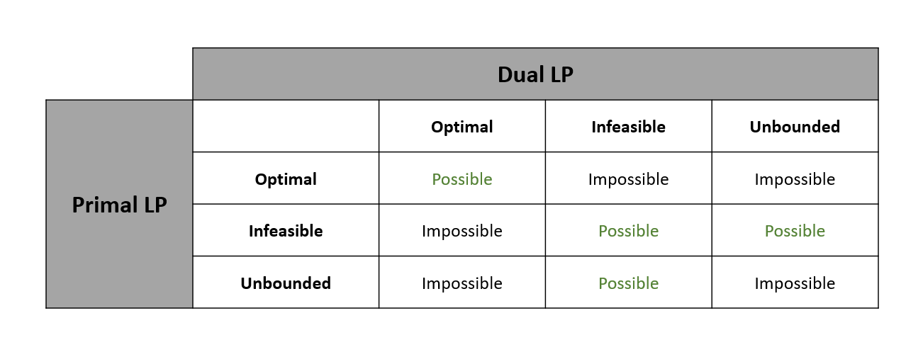
Using Duality to Determine Feasibility & Boundedness of LP
- Infeasible: there is no point that satisfies the constraints
- Feasible & Bounded (Optimal): there is a feasible point of maximum objective function value
- Feasible & Unbounded: there are feasible points of arbitrarily large value

Example: 2-Player Zero Sum Game
References
[ ] how to calculate solution for LP (simplex method)
[ ] how to prove duality
[ ] how to prove optimal solution for shortest path problem